Overview
This guide shows how to build custom stock and crypto candlestick charts in Python with mplfinance. You’ll learn quick setup, practical customization (indicators, styles, panels), and how to keep plots fast for algorithmic trading workflows.
Quickstart
- Requirements: Python 3.9+, pandas, numpy, mplfinance (optionally yfinance for data).
pip install mplfinance pandas numpy yfinance
Minimal steps:
- Fetch OHLCV data into a pandas DataFrame with a DatetimeIndex.
- Ensure columns: Open, High, Low, Close, Volume.
- Call mpf.plot with your options.
import yfinance as yf
import mplfinance as mpf

# Example: crypto daily candles
df = yf.download('BTC-USD', period='180d', interval='1d')
# Keep only required columns, drop NAs
df = df[['Open','High','Low','Close','Volume']].dropna()

mpf.plot(
    df,
    type='candle',
    volume=True,
    mav=(20,50),
    style='yahoo',
    title='BTC-USD — 180D'
)
Minimal Working Example (no network)
Generate synthetic OHLCV and plot a candlestick with moving averages and volume.
import numpy as np
import pandas as pd
import mplfinance as mpf

np.random.seed(7)
idx = pd.date_range('2024-01-01', periods=80, freq='D')
close = pd.Series(100 + np.cumsum(np.random.randn(len(idx))*1.2), index=idx)
open_ = close.shift(1).fillna(close.iloc[0])
high = pd.concat([open_, close], axis=1).max(axis=1) + np.random.rand(len(idx))
low = pd.concat([open_, close], axis=1).min(axis=1) - np.random.rand(len(idx))
vol = (3e5 + np.random.rand(len(idx))*2e5).astype(int)

df = pd.DataFrame({
    'Open': open_, 'High': high, 'Low': low, 'Close': close, 'Volume': vol
})

mpf.plot(df, type='candle', volume=True, mav=(10,20), title='Synthetic OHLCV')
Core Steps for Custom Charts
- Load data
- Use yfinance, exchange APIs, or CSVs; ensure DatetimeIndex.
import pandas as pd
# Example CSV must contain Date,Open,High,Low,Close,Volume
# df = pd.read_csv('data.csv', parse_dates=['Date'], index_col='Date')
- Choose plot type
- type='candle' or 'ohlc' for bars; 'line' for closes; 'renko'/'pnf' also supported.
- Add overlays and indicators
- Moving averages, Bollinger Bands, RSI, VWAP, custom signals with addplot().
- Style the chart
- Use built-ins (e.g., 'yahoo', 'charles') or customize market colors.
- Export or embed
- savefig='file.png' or returnfig=True to integrate with apps.
Useful Arguments at a Glance
| Argument | Purpose | Example |
|---|---|---|
| type | chart type | candle, ohlc, line |
| volume | show volume panel | volume=True |
| mav | moving average(s) | mav=(20,50) |
| style | theme | style='yahoo' |
| addplot | extra series/panels | list of mpf.make_addplot |
| panel_ratios | main/indicator heights | panel_ratios=(3,1) |
| figscale | overall size | figscale=1.2 |
| savefig | save to file | savefig='chart.png' |
Practical Customization
Indicators (Bollinger Bands + RSI), custom colors, and trade markers.
import numpy as np
import pandas as pd
import yfinance as yf
import mplfinance as mpf
# Download stock candles
sym = 'AAPL'
df = yf.download(sym, period='6mo', interval='1d')
df = df[['Open','High','Low','Close','Volume']].dropna()
# Indicators
close = df['Close']
mavg = close.rolling(20).mean()
std = close.rolling(20).std()
upper = mavg + 2*std
lower = mavg - 2*std
def rsi(s, period=14):
delta = s.diff()
gain = delta.clip(lower=0).rolling(period).mean()
loss = (-delta.clip(upper=0)).rolling(period).mean()
rs = gain / loss
return 100 - (100 / (1 + rs))
r = rsi(close)
# Example trade markers (toy signals)
buys = pd.Series(np.nan, index=df.index)
sells = pd.Series(np.nan, index=df.index)
mask_b = close > mavg
mask_s = close < mavg
buys[mask_b] = df['Low'][mask_b] * 0.995
sells[mask_s] = df['High'][mask_s] * 1.005
ap = [
mpf.make_addplot(mavg, color='dodgerblue'),
mpf.make_addplot(upper, color='grey'),
mpf.make_addplot(lower, color='grey'),
mpf.make_addplot(r, panel=1, color='purple', ylabel='RSI', ylim=(0,100)),
mpf.make_addplot(buys, type='scatter', marker='^', markersize=60, color='g'),
mpf.make_addplot(sells, type='scatter', marker='v', markersize=60, color='r'),
]
mc = mpf.make_marketcolors(up='green', down='red', inherit=True)
style = mpf.make_mpf_style(base_mpf_style='yahoo', marketcolors=mc)
mpf.plot(
df,
type='candle',
addplot=ap,
volume=True,
style=style,
panel_ratios=(3,1),
figscale=1.2,
title=f'{sym} — Custom Bands, RSI, Trade Marks'
)
Crypto vs. Stocks: Data Considerations
- Trading hours: Stocks skip weekends/overnights; crypto is 24/7. For intraday stocks, compressed time is expected; for crypto, data is continuous.
- Index timezone: Normalize to one timezone across feeds. If needed: df.tz_localize(None) or df.tz_convert('UTC').
- Intervals: Use consistent bars before merging indicators or signals.
Performance Notes
- Plot fewer rows: df.iloc[-1000:] for a fast, focused chart window.
- Resample before plotting: e.g., 1-minute to 5-minute to reduce candles.
# Resample 1-minute crypto to 5-minute
agg = {
    'Open': 'first', 'High': 'max', 'Low': 'min', 'Close': 'last', 'Volume': 'sum'
}
df_5m = df.resample('5T').apply(agg).dropna()
- Limit overlays: Heavy addplots and large markers slow rendering.
- Use simpler styles and avoid excessive transparency.
- Precompute indicators once; do not recompute inside plotting loops.
- Batch-export: Reuse figures with returnfig=True when generating many charts.
fig, axes = mpf.plot(df.iloc[-300:], type='candle', returnfig=True)
# ... draw additional elements via matplotlib if needed ...
Common Pitfalls
- Wrong columns: Ensure exactly Open, High, Low, Close, Volume (case-sensitive).
- Non-DatetimeIndex: Convert with parse_dates and set index_col.
- NaNs in OHLC: Fill or drop before plotting to avoid gaps or errors.
- Timezone mismatch: Align tz across data sources to keep joins and panels correct.
- Inconsistent frequency: Mixing 1D with 1H data will misalign indicators.
Save and Share
mpf.plot(df.iloc[-200:], type='candle', volume=True, style='charles', savefig='chart.png')
Tiny FAQ
- How do I add a secondary indicator panel? Use make_addplot(..., panel=1) and set panel_ratios.
- Can I plot only a date range? Slice by index: df.loc['2024-05-01':'2024-08-31'].
- How do I change up/down colors? Use make_marketcolors and make_mpf_style.
- Does mplfinance handle live updates? It’s primarily static; generate frames or redraw periodically.
- Is log scale supported? Use line plots on transformed data or pre-transform before plotting.